10 Excel Functions You Need to Know for Data Analysis

Adept’s resident Excel Nerd is back with her second post covering Excel implementation. Here are 10 must-know functions for data analysis, plus some additional tips & tricks.

Just yesterday, I was in a conversation with some coworkers discussing a process that could be very time consuming, and how to handle it. I realized within a minute that a combination of Excel functions and automated Supermetrics data pulls could cut the time by at least half. I explained the other options and we quickly came up with a better process. Scenarios like this happen all the time and can be solved by some basic function knowledge.

All SEOs, and marketers in general, should know how powerful Excel is—and when to realize that a function or feature could save them hours of time. I’m not saying you need to have them memorized (I Google functions all the time!), but realizing when you should utilize Excel is a key skill to help you work efficiently and improve your job worth.

It’s hard for me to pick my favorite Excel functions, but there are some I definitely use more than others. If you are brand new to excel, check out the basics of excel here. Knowing these functions has helped me save time  and improve internal processes, and I want to help you do that as well.

I’ve created a training Excel document to go along with each function. Each has example problems, the solution, and a place to try yourself. Download it at the bottom of this blog post, or here. Remember, these are examples; there are many different ways you could utilize them in the real world.

10 Excel Functions for Data Analysis:

1. Concatenation
2. Len
3. Find & Replace
4. Filter & Sort
5. Conditional Formatting
6. Index Match
7. Remove Duplicates
8. Logic Functions
9. IfError
10. Short Cuts and Tips

1. Concatenation

Simply put, concatenation combines different text into one cell. Add a domain name to a URL slug, create rules for title tags, build API queries, and automate JSON schema quicker than ever before.

=concatenate(text1,text2,…)

I could go on and on about the uses for concatenation, but why do that when Annie Cushing has already done the hard work with 21 Real-World Examples Of Concatenating Marketing Data In Excel? Read it, learn it, use it.

2. LEN

LEN is simple. It returns the number of characters in another cell. Use LEN when creating title tags or descriptions that have character limits, and you’ll immediately know if your text might be truncated.

=LEN(A1)

Of course, Google has changed the rules and shown different limits in SERPs depending on the search query, but with best practices, the use of LEN will never go away.

3. Find & Replace

Find and replace has recently become a go-to function for me, and it seems like many people forget about it. It does exactly what it sounds like: finds text, and replaces it with other text that you specify.

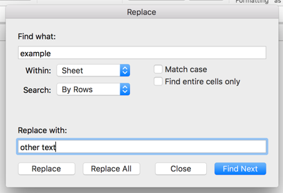
Some uses:

• Remove Adwords markup on a list of keywords so SEO can utilize them easier
• Replace all references to a past month and update to current month in a report
• Update a list of folder structures for a redirect plan
• Update part of title tags or meta descriptions in bulk
• Change HTTP to HTTPS on a list of URLS
• Remove extra spaces or an incorrect brand name in a list

4. Filter & Sort

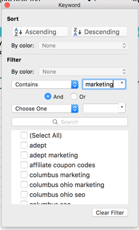
Filter and sort are fairly common Excel features, but I wanted to include these and talk about how to use them to prioritize SEO tasks. Sometimes SEO can become overwhelming, and data needs to be paired down in order to prioritize. Filter and sort are helpful with these.

Filtering is specifically useful when looking at a list of data and organizing by common terms. Take a list of keywords and filter by how many have contain similar topic keywords:

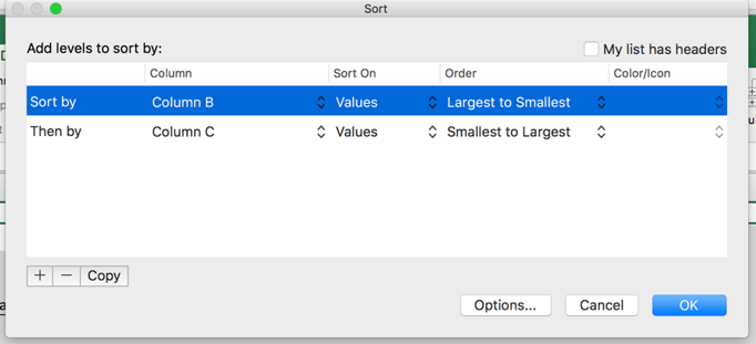
Sorting is useful when prioritizing a list by highest values or lowest values. Sort landing pages by lowest conversion rate, highest revenue, or highest number of sessions to prioritize where to focus different efforts to improve. Use advanced sorting as well – where you can sort by what keywords have the highest search volume and lowest competition, or landing pages that have highest sessions but lowest conversion rate.

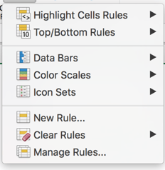
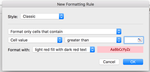
5. Conditional Formatting

I cannot stress enough how important conditional formatting is when analyzing or reporting data. Use it to highlight good data, bad data, % change, top search volume keywords, duplicate values, and so many more. Spend some time going through all the conditional formatting rules to understand how powerful it truly is.

6. Index & Match

You may have heard of lookups before. Vlookup was a go-to for me for quite a while, but it has some limitations that could give you the wrong data if you’re not careful.

Then, I found another Annie Cushing blog post that changed everything – with a helpful video tutorial of how to use index match instead of lookups. It took me a few months to get used to using it, but now I can’t live without it.

Index and match by themselves are useful functions, but together they should be your number one when combining data sources. Here’s a high level overview of what the functions look like together:

=INDEX(B:B,Match(A1,A:A,0))

And a simplified explanation of the function:

=INDEX(Column of Data You Want to Return,MATCH(Common Data Point You are trying to Match, Column of Other Data Source that has Common Data Point,0))

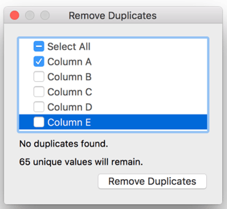
7. Remove Duplicates

SEOs, and marketers in general, spend a lot of time combining many data sources and pieces of information. Keyword research is a great example. I may use 5+ different data sources to pull keyword ideas, and some of these have overlapping keywords. Use the built-in function to remove the duplicates.

Simply highlight the data you want to remove. Be sure to include the whole data set, and select only the column you want to remove the duplicates in. You have other columns of data mapped to the duplicates that you don’t want to screw up.

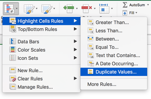
To get a visual of how many there are, use conditional formatting to highlight the duplicates first:

Pro tip – Remove duplicates keeps the first unique cell in the column. If you have data you want to keep in another column for one of the duplicates more than the other, sort by those values first, then remove the duplicates. 

8. Logic Functions

Logic functions seem like they are difficult to use, but they make sense if you really think about them. There are a handful of logic functions that are  very useful for marketing.

Logic functions ask a question of the data. If the result is true, you return one specified result. If the result is false, you return another. For example, you can ask the data to sum only the data if it’s greater than 100 or average only the data that is less than 10. A more complex example could be to multiply the data by X if it’s less than 3 and multiply the data by Y if It’s more than 3.

You can add onto these as much as you want and create nested functions, but the more you do, the more overwhelming the logic can become.

Sticking to the simple logic functions is fine for now: 

=IF(logical_test,value_if_true,value_if_false) – simple explanation from excel: IF(Something is True, then do something, otherwise do something else) 

=AND(logical1,logical2,…) – Utilize this with the If function to create multiple two or more logic rules that occur together

=OR(logical1,logical2,…) – Utilize this with the If function to create multiple scenarios

=SUMIF(range,criteria,sum_range) – Sums a range that follows a specified criteria. The criteria range and sum range can be different, but must have the same size range.

=SUMIFS(sum_range1,criteria_range1,criteria1,…) – Sums multiple ranges based on multiple specified criteria. Each criteria and sum range can be different. Note the difference in syntax from the sumif.

=AVERAGEIF(range,criteria,average_range)  – Averages a range that follows a specified criteria. The criteria range and sum range can be different, but must have the same size range.

=AVERAGEIFS(average_range1,criteria_range1,criteria1,…) – Averages multiple ranges based on multiple specified criteria. Each criteria and average range can be different. Note the difference in syntax from the averageif. 

=COUNT(value1,value2,…) – Counts number of cells with numbers in them.

=COUNTA(value1,value2,…) – Just like Count, but returns count of text cells.

=COUNTBLANK(range) – Returns count of blank cells.

=COUNTIF(range,criteria) – Returns count of cells that follow a specified rule.

=COUNTIFS(criteria_range1,criteria,…) – Returns count of cells that follow multiple specified criteria.

9. IfError

Ever end up with the ugly “#N/A” error and it drives you nuts? Iferror is a function blessing and able to clean those up in a second! Just wrap any function in iferror as the value, and enter the response you would like to return if there is an error:

=IFERROR(value,value_if_error)

I use this for combining data sources and data points that are missing in the other data source. For example, when combing GA data with a keyword export and there is no GA data for one of the ranking URLS, if you want to return an empty cell instead just insert two quotations. You can change the error response to “no data,” or whatever you prefer.

=IFERROR(index(B:B,match(A1,A:A,)),””)

=IFERROR(index(B:B,match(A1,A:A,)),”No Data”) 

Special shout out to all professors that waited until the very last semester of college to tell me about iferror. Still think about all the time it could have saved me if I knew about it sooner.

10. Short-Cut Functions & Tips

There are plenty of other functions and short cuts that don’t need to be covered in depth, but are still some of my favorites to use: 

• Proper(A1) – Uppercase every word in the text
• Lower(A1) – lowercase all text
• Upper(A1) – Uppercase all text
• Trim(A1) – Removes odd spacing around text
• ISBLANK(A1) – Identifies if the cell is blank and returns a Yes or No
• Add a ‘ to the start of your function to lock it in text mode mid-function to not create an error if you have to come to back to it.
• Paste Special - Values Only in order to remove the functions from your data so you can work on it without potentially screwing up the formulas.
• Lock cells within a function with a shortcut:
  • Mac – Command T
  • PC – F4 
  • $A$1 – entire cell is locked and won’t change if you drag the function
  • $A1 – Column is locked but row will change if you drag the function
  • A$1 – Row is locked but column will change if you drag the function
• Modifiers

I used Excel a lot in college, and always struggled with the lack of real world examples to understand when to apply a lot of functions. I don’t want you to struggle with that as well. Take a look at some of the sample problems I created and give it a shot, and hopefully you’ll improve your own Excel knowledge!

I kept this post limited to the simple functions and features everyone should know. I’ll be getting more in-depth with specific how-to’s with future posts (check out my first Excel post about customizing data here). Stay tuned, share this post on Twitter, and let me know in the comments if I’ve missed a key function, or if you have questions on the spreadsheet!